Create a Multimodal GTA-V RAG application

Artificial Intelligence (AI) has been actively working with text for quite some time, but the world isn’t solely centered around words. If you take a moment to look around, you’ll find a mix of text, images, videos, audios, and their combinations.

Today we are going to work on Multimodality which is basically a concept that essentially empowers AI models with the capacity to perceive, listen, and comprehend data in diverse formats together with the text. Pretty much like how we do!

In an ideal situation, we should be able to mix different types of data together and show them to a generative AI model at the same time and iterate on it. It could be as simple as telling the AI model, “Hey, a few days ago, I sent you a picture of a brown, short dog. Can you find that picture for me?” and the model should then give us the details of that picture. Basically, we want the AI to understand things more like how we humans do, becoming really good at handling and responding to all kinds of information.

But the challenge here is to make a computer understand one data format with its related reference, and that could be a mix of text, audio, thermal imagery, and videos. Now to make this happen, we use something called Embeddings. It’s really a numeric vector which contains a bunch of numbers written together that might not mean much to us but are understood by machines very well.

Cat is equal to Cat

Let’s think of the text components for now, so we are currently aiming that our model should learn that words like “Dog” and “Cat” are closely linked to the word “Pet.” Now this understanding is easily achievable by using an embedding model which will convert these text words into their respective embeddings first and then the model is trained to follow a straightforward logic: if words are related, they are close together in the vector space, if not, they would be separated by the adequate distance.

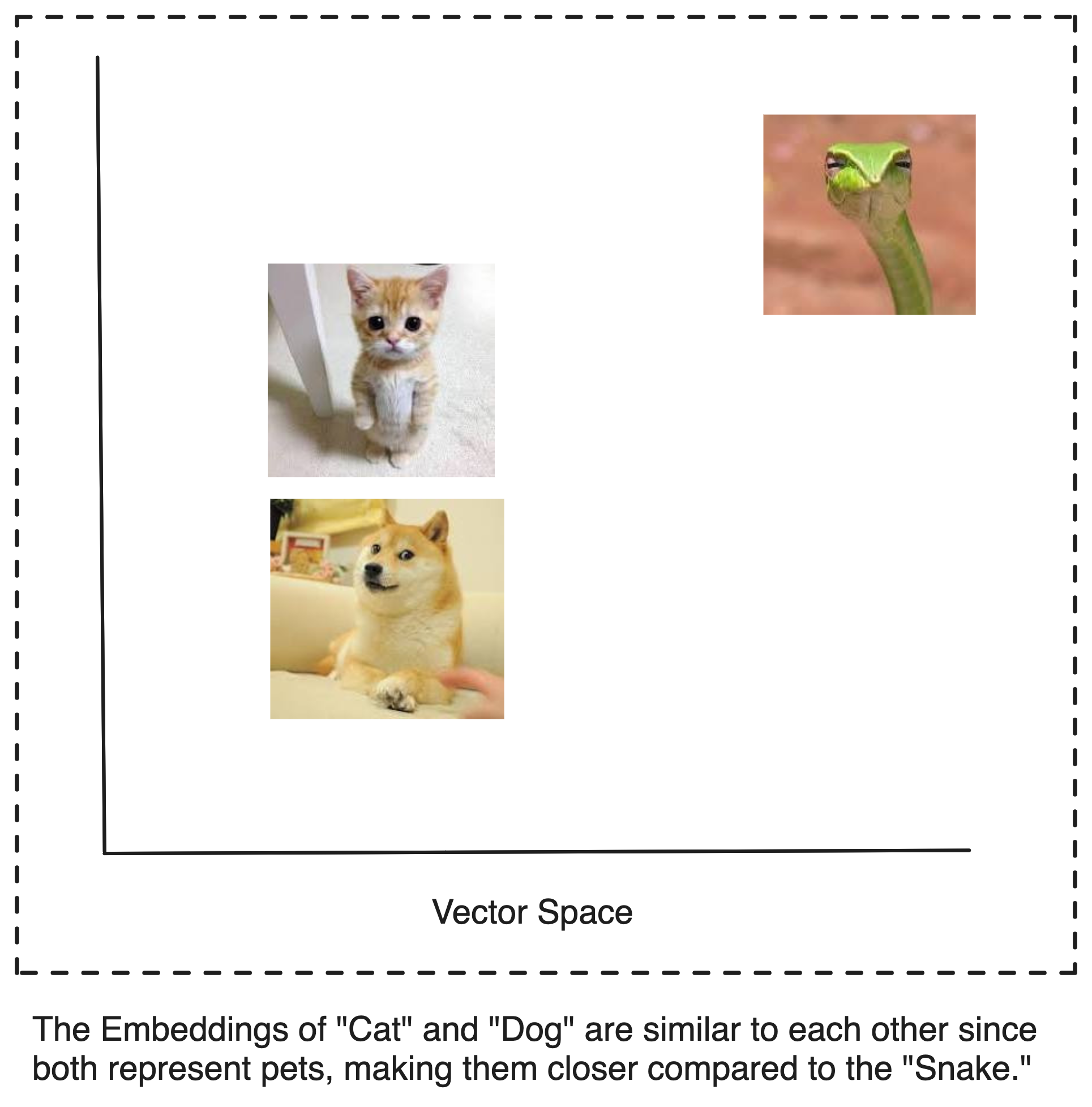
But to help a model recognize that an image of a “Cat” and the word “Cat” are similar, we rely on Multimodal Embeddings. To simplify things a bit, imagine there is a magic box which is capable of handling various inputs – images, audios, text, and more.

Now, when we feed the box with an image of a “Cat” with the text “Cat,” it performs its magic and produces two numeric vectors. When these two vectors were given to a machine, it made machines think, “Hmm, based on these numeric values, it seems like both are connected to “Cat”. So that’s exactly what we were aiming for! Our goal was to help machines to recognize the close connection between an image of a “Cat” and the text “Cat”. However, to validate this concept, when we plot those two numeric vectors in a vector space, it turns out they are very close to each other. This outcome exactly mirrors what we observed earlier with the proximity of the two text words “Cat” and “Dog” in the vector space.

Ladies and gentlemen, that’s the essence of Multimodality. 👏

So we made our model to comprehend the association between “Cat” images and the word “Cat.” Well this is it, I mean if you are able to do this, you would have ingested the audio, images, videos as well as the word “Cat” and the model will understand how the cat is being portrayed across all kinds of file format..

RAG is here..

Well if you don’t know what RAG means, I would highly advise you to read this article here which I wrote some days back and loved by tons of people, not exaggerating it but yeah, it’s good to get the balls rolling..

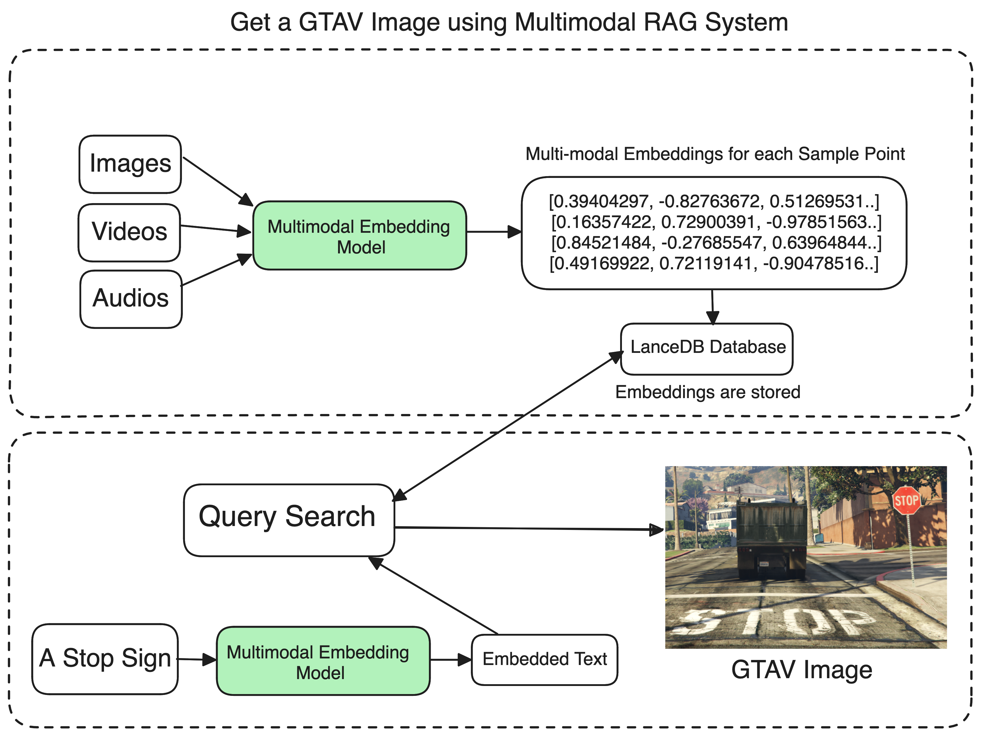
So there are impressive models like DALLE-2 that provide text-to-image functionality. Essentially, you input text, and the model generates relevant images for you. But can we create a system similar to Multimodal RAG, where the model produces output images based on our own data? Alright, so the goal for today is to create an AI model that when asked something like, “How many girls were there in my party?” 💀 not only provides textual information but also includes a relevant image related to it. Think of it as an extension of a simple RAG system, but now incorporating images.

Before we dive in, remember that Multimodality isn’t limited to just text-to-image or image-to-text as it encompasses the freedom to input and output any type of data. However, for now, let’s concentrate on the interaction from image to text exclusively.

Contrastive learning

Now the question is, What exactly was that box doing? The magic it performs is known as Contrastive Learning. While the term might sound complex, it’s not that tricky. To simplify, consider a dataset with images, along with a caption describing what the image represents.

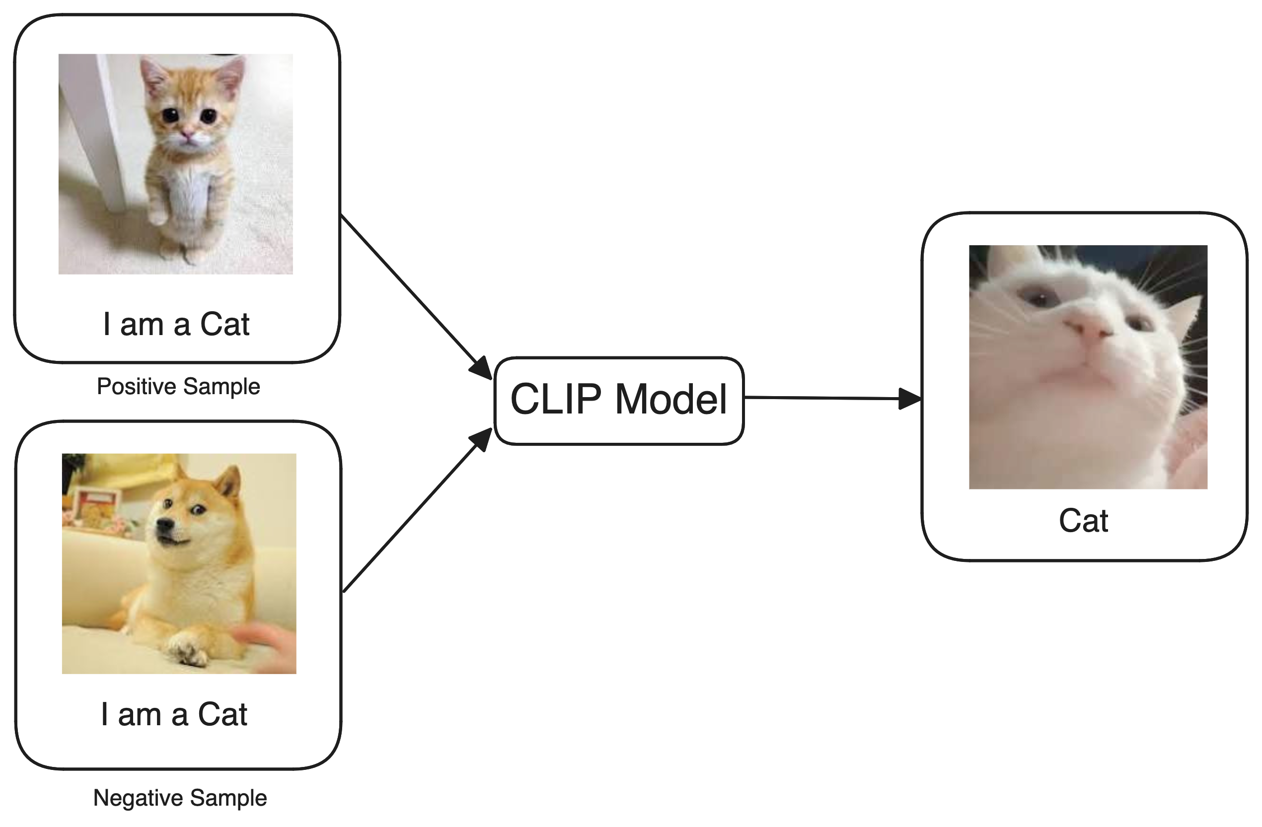
Alright, now what happens is: we give our text-image model with these Positive and Negative samples, where each sample consists of an image and a descriptive text. Positive samples are those where the image and text are correctly aligned – for instance, a picture of a cat matched with the text “this is an image of a cat.” Conversely, negative samples involve a mismatch, like presenting an image of a dog alongside the text “this is an image of a cat.”

Now we train our text-image model to recognize that positive samples offer accurate interpretations, while negative samples are misleading and should be disregarded during training. In formal terms this technique is called CLIP (Contrastive Language-Image Pre-training) introduced by OpenAI where authors trained an image-text model on something around 400 million image caption pairs taken from the internet and everytime model makes a mistake, the contrastive loss function increases and penalize it to make sure the model trains well. The same kind of principles are applied to the other modality combinations as well, so the voice of cat with the word cat is a positive sample for speech-text model, a video of cat with the descriptive text “this is a cat” is a positive sample for video-text model.

Show time

Well you don’t have to build that box from scratch because folks have already done it for us. There’s a Multimodal embedding model, like the “ViT-L/14” from OpenAI. This model can handle various data types, including text, images, videos, audios, and even thermal and gyroscope data. Now, onto the next question: how do we store those embeddings?

For that we’ll need a vector database that can efficiently fetch, query, and retrieve relevant embeddings for us, ideally one that supports multimodal data and doesn’t burn a hole in our wallets. That’s where LanceDB comes into play.

Vector database

When we talk about the vector database, there are ton of options available in the current market, but there is something about the LanceDB which makes it stands out as an optimal choice for a vector database, As far as I have used it, it address the limitations of traditional embedded databases in handling AI/ML workloads. When I say traditional, it typically means those database management tools which are not aligned with the usage of heavy computation that comes with the ML infra.

TLDR; LanceDB operates on a serverless architecture, meaning storage and compute are separated into two distinct units. This design makes it exceptionally fast for RAG use cases, ensuring fast fetching and retrieval. Additionally, it has some notable advantages – being open source, utilizing its Lance columnar data format built on top of Apache Arrow for high efficiency, persistent storage capabilities, and incorporating its own Disk Approximate Nearest Neighbor search. All these factors collectively make LanceDB an ideal solution for accessing and working with multimodal data. I love you LanceDB ❤️.

Data time

To add some excitement, I’ve crafted a GTA-V Image Captioning dataset, featuring thousands of images, each paired with a descriptive text illustrating the image’s content. Now, when we train our magic box, the expectation is clear – if I ask that box to provide me an image of “road with a stop sign,” it should deliver a GTA-V image of a road with a stop sign on it. Otherwise, what’s the point, right?

FAQ

1. We will be using “ViT-L/14” to convert our multimodal data into its respective embeddings.
2. LanceDB as our vector database to store the relevant embeddings.
3. GTA-V Image Captioning dataset for our magic box.

Environment Setup

I am using a MacBook Air M1, and it’s important to note that some kinds of dependencies and configurations may vary depending on the type of system that you are running, so it’s important to take that into account.

Here are the steps to install the relevant dependencies

# Create a virtual environment
python3 -m venv env

# Activate the virtual environment
source env/bin/activate

# Upgrade pip in the virtual environment
pip install --upgrade pip

# Install required dependencies
pip3 install lancedb clip torch datasets pillow 
pip3 install git+https://github.com/openai/CLIP.git

And don’t forget to get your access token from the hugging face to download the data.

Downloading the Data

Dataset can easily be fetched using the datasets library.

import clip
import torch
import os
from datasets import load_dataset

ds = load_dataset("vipulmaheshwari/GTA-Image-Captioning-Dataset")
device = torch.device("mps")
model, preprocess = clip.load("ViT-L-14", device=device)

Downloading the dataset may require some time, so please take a moment to relax while this process completes. Once the download is finished, you can visualize some sample points like this:

from textwrap import wrap
import matplotlib.pyplot as plt
import numpy as np

def plot_images(images, captions):
    plt.figure(figsize=(15, 7))
    for i in range(len(images)):
        ax = plt.subplot(1, len(images), i + 1)
        caption = captions[i]
        caption = "\n".join(wrap(caption, 12))
        plt.title(caption)
        plt.imshow(images[i])
        plt.axis("off")

# Assuming ds is a dictionary with "train" key containing a list of samples
sample_dataset = ds["train"]
random_indices = np.random.choice(len(sample_dataset), size=2, replace=False)
random_indices = [index.item() for index in random_indices]

# Get the random images and their captions
random_images = [np.array(sample_dataset[index]["image"]) for index in random_indices]
random_captions = [sample_dataset[index]["text"] for index in random_indices]

# Plot the random images with their captions
plot_images(random_images, random_captions)

# Show the plot
plt.show()

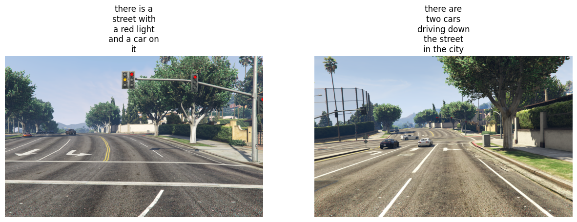
Storing the Embeddings

The dataset consists of two key features: the image and its corresponding descriptive text. Initially, our task is to create a LanceDB table to store the embeddings. This process is straightforward – all you need to do is define the relevant schema. In our case, the columns include “vector” for storing the multimodal embeddings, a “text” column for the descriptive text, and a “label” column for the corresponding IDs.

import pyarrow as pa
import lancedb
import tqdm

db = lancedb.connect('./data/tables')
schema = pa.schema(
  [
      pa.field("vector", pa.list_(pa.float32(), 512)),
      pa.field("text", pa.string()),
      pa.field("id", pa.int32())
  ])
tbl = db.create_table("gta_data", schema=schema, mode="overwrite")

Executing this will generate a table with the specified schema, and it’s ready to store the embeddings along with the relevant columns. It’s as straightforward as that – almost too easy!

Encode the Images

Now, we’ll simply take the images from the dataset, feed them into an encoding function that leverages our Multimodal Embedding model, and generate the corresponding embeddings. These embeddings will then be stored in the database.

def embed_image(img):
    processed_image = preprocess(img)
    unsqueezed_image = processed_image.unsqueeze(0).to(device)
    embeddings = model.encode_image(unsqueezed_image)
    
    # Detach, move to CPU, convert to numpy array, and extract the first element as a list
    result = embeddings.detach().cpu().numpy()[0].tolist()
    return result

So our embed_image function takes an input image, prepocesses it through our CLIP model preprocessor, encode the preprocessed image and returns a list representing the embeddings of that image. This returned embedding serves as a concise numerical representation, capturing all the key features and patterns within the image for downstream tasks or analysis. The next thing is to call this function for all the images and store the relevant embeddings in the database.

data = []
for i in range(len(ds["train"])):
    img = ds["train"][i]['image']
    text = ds["train"][i]['text']
    
    # Encode the image
    encoded_img = embed_image(img)
    data.append({"vector": encoded_img, "text": text, "id" : i})

Here, we’re just taking a list, adding the numeric embeddings, reference text and the current index id to it. All that’s left is to include this list in our LanceDB table. And voila, our datalake for the embeddings is set up and good to go!

tbl.add(data)
tbl.to_pandas()

Up until now, we’ve efficiently converted the images into their respective multimodal embeddings and stored them in the LanceDB table. Now the LanceDB tables offer a convenient feature: if there’s a need to add or remove images, it’s remarkably straightforward. Just encode the new image and add it, following to the same steps we followed for the previous images.

Query search

Our next move is to embed our text query using the same multimodal embedding model we used for our images. Remember that “box” I mentioned earlier? Essentially, we want this box to create embeddings for both our images and our texts which ensures that the representation of different types of data happens in the same way. Following this, we just need to initiate a search to find the nearest image embeddings that matches our text query.

def embed_txt(txt):
    tokenized_text = clip.tokenize([txt]).to(device)
    embeddings = model.encode_text(tokenized_text)
    
    # Detach, move to CPU, convert to numpy array, and extract the first element as a list
    result = embeddings.detach().cpu().numpy()[0].tolist()
    return result

res = tbl.search(embed_txt("a road with a stop")).limit(3).to_pandas()
res

0 | [0.064575195, .. ] | there is a stop sign...| 569 |	131.995728
1 | [-0.07989502, .. ] | there is a bus that... | 423 | 135.047852
2 | [0.06756592, .. ]  | amazing view of a ...	| 30  | 135.309937

Let’s slow down a bit and understand what just happened. Putting simply, the code snippet executes a search algorithm in its core to pinpoint the most relevant image embedding that aligns with our text query. The resulting output, as showcased above, gives us the embeddings which closely resembles our text query. In the result, the second column presents the embedding vector, while the third column contains the description of the image that closely matches our text query. Essentially, we’ve determined which image closely corresponds to our text query by examining the embeddings of both our text query and the image.

It’s similar to saying, If these numbers represent the word “Cat”, I spot an image with a similar set of numbers, so most likely it’s a match for an image of a “Cat”. 😺

If you are looking for the explanation of how the search happens, I will write a detailed explanation in the coming write ups because it’s so exciting to look under the hood and see how the searching happens. Essentially there is something called Approximate Nearest Neighbors (ANN) which is a technique used to efficiently find the closest points in high-dimensional spaces. ANN is extensively used in data mining, machine learning, computer vision and NLP use cases. So when we passed our embedded text query to the searching algorithm and asked it to give us the closest sample point in the vector space, it used a type of ANN algorithm to get it for us. Specifically LanceDB utilizes DANN (Deep Approximate Nearest Neighbor) for searching the relevant embeddings within its ecosystem..

In our results, we have five columns. The first is the index number, the second is the embedding vector, the third is the description of the image matching our text query, and the fourth is the label of the image. However, let’s focus on the last column – Distance. When I mentioned the ANN algorithm, it simply draws a line between the current data point (in our case, the embedding of our text query) and identifies which data point (image embedding) is closest to it. If you observe that the other data points in the results have a greater distance compared to the top one, it indicates they are a bit further away or more unrelated to our query. Just to make it clear, the calculation of distance is a part of the algorithm itself.

D-DAY

Now that we have all the necessary information, displaying the most relevant image for our query is straightforward. Simply take the relevant label of the top-matched embedding vector and showcase the corresponding image.

data_id = int(res['id'][0])
display(ds["train"][data_id]['image'])
print(ds["train"][data_id]['text'])

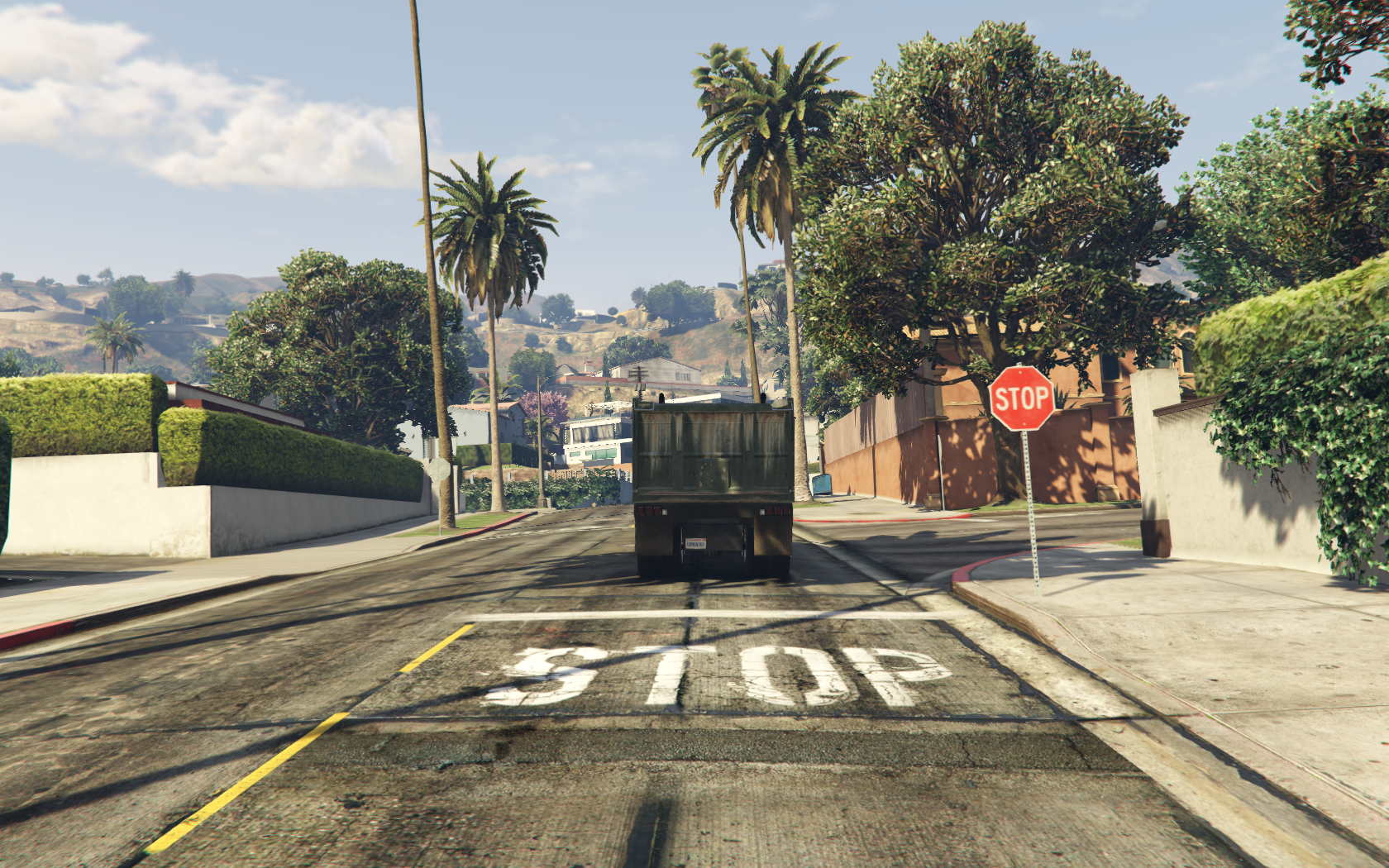
there is a truck driving down a street with a stop sign

What’s next?

To make things more interesting, I’m currently working on creating an extensive GTA-V captioning dataset. This dataset will include a larger number of images paired with their respective reference text, providing us with a richer set of queries to explore and experiment with.. Nevertheless, there’s always room for refining the model. We can explore creating a customized CLIP model, adjusting various parameters. Increasing the number of training epochs may afford the model more time to grasp the relevance between embeddings. Additionally, there’s an impressive multimodal embedding model developed by the Meta known as ImageBind. We can consider trying ImageBind as an alternative to our current multimodal embedding model and compare the outcomes. With numerous options available, the fundamental concept behind the Multimodal RAG workflow remains largely consistent.

Here’s how everything comes together in one frame and this is the Collab for your reference